Comments on Value-at-Risk (VaR)

• Value-at-risk (VaR) answers the question: "how bad things can be in terms of investment losses?"
• VaR can be calculated by at least two methods: historical analysis and Monte Carlo simulations;
• Mathematical definition and comments on backtesting of a VaR model.

Hello all!

Last post, I have discussed a significant risk factor when investing in derivatives, named volatility risk. In this post, I would like to continue discussing topics related to risk measurement, this time focusing on the calculation of VaR (value-at-risk) which is an important metric in portfolio management. 

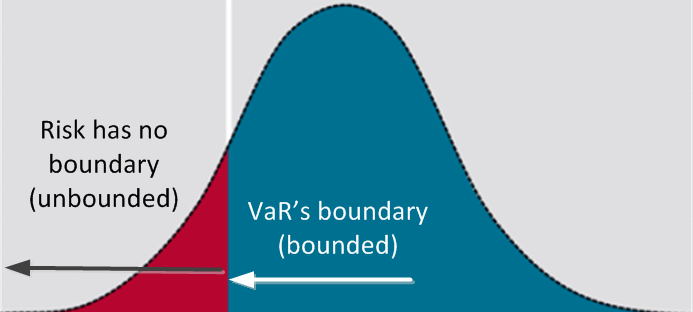
The idea behind it is in fact simple. The associated idea is to provide the maximum possible loss within a determined confidence level. This way one can say something like "95% that the maximum loss is 4% in the next day". Put in other words, it means that we are 95% sure that the return of a determined portfolio (with one or several assets) in the end of the next day will be between -4% and "infinite". This "infinite" sounds weird, but it is because VaR is associated with loss risk so the integration begins in positive infinite down to a value that guarantees the required confidence. Other metric should provide the profit potential (although statistically the discussion doesn't change, only the point of view).

There are least two ways to calculate VaR that I will discuss here. The first is by means of historical data and the second is by Monte Carlo simulations (other methods for example in this introductory paper). As already discussed in another post (Data driven and market driven models), these two approaches actually represents two different assumptions with respect to the expectation on the future movements of the market. When using historical data, the implicit assumption is that past events can somehow be a good proxy for the results in the next future period. On the other hand, Monte Carlo simulations take a stochastic differential equation or more directly the assumed probability distribution as the indicator for the future movements. In this case, the parameters of the models used for MC simulations can be acquired from market data.

Mathematical definitions

Consider a portfolio with $n$ assets, $V=\{S_1, S_2, S_3, ..., S_n\}$. The value of this portfolio at $t$ will be given by $V(t)= \sum_i S_i(t)$. Suppose one needs to calculate the value-at-risk within a time horizon $\alpha$ with a confidence level $p$. The expected return of the portfolio at $t+\alpha$ would be given by $E_P[ \frac{V(t+\alpha)-V(t)}{V(t)} |\Theta(t)]$ where the expectation is calculated within the real-world measure denoted by $P$, and $\Theta(t)$ denotes the filtration at time $t$. In the expectation calculation, one considers a joint probability encompassing all assets included in the portfolio. Denote $F(\delta V)$ as the cumulative probability function (CDF) associated with the joint probability $P(\delta V)$, where $\delta V$ is the return of the portfolio within the time horizon $\alpha$. Therefore, the value-at-risk (VaR) within a time horizon $\alpha$ and with a confidence level $p$ is given by:

$VaR = inf  \{ y | F(y) \leq (1-p) \}$

where $inf\{\}$ denotes the lower value.

Historical approach

As seen in the section above, the first significant input for VaR calculation is the return probability function. This input will provide us the weight that each possible return value has. Let's take a look in how to obtain this probability from historical data.

For sake of simplicity, we focus on a single asset in the portfolio. It could be a stock, for instance. In this simplest approach, we take a list of recent historical quotes per day. For each day we calculate the return with respect to the previous day. If we assume that every day in this historical set is worth equal, we then build a frequency plot and obtain a probability density by normalization and fitting of this plot. Some more elaborated models can be based on a weighted consideration of the daily returns. Put in other others, return values that happened in a relative long time ago could have lower weight than a return that happened only a week ago. In this case, one can simply elaborated the frequency plot weighting the contribution of each return by the respective "relevance" coefficient according to the model.
Now consider the case we add several assets in the evaluated portfolio. When dealing with several assets, the correlation among them plays a role in the joint return probability. In the simplest historical approach, one can skip complications with correlations by evaluating the historical return of the entire portfolio (as it is by now, that is, asset quantities remain the same for the whole historical period). In this case, one ends up with a single return probability distribution that (supposedly) holds for the portfolio.
Here an observation is due. Once dealing with a joint probability distribution, one may needs a considerable longer historical data analysis in order to obtain a convergence in the probability distribution.

Playing dices -- Monte Carlo simulations

Calculation of VaR through historical data analysis is simple and non-parametric, that is, there is no previous assumptions about what the probability distribution could look like. Despite the simplicity, some strong assumptions are the weaknesses of the method. For instance, historical data analysis consider that future is a repetition of the past distribution. There is no guarantee of this assumption at all.
A well-known alternative method is the use of Monte Carlo simulations to get the portfolio return distribution. In principle, the Monte Carlo idea is to get average behavior by brute force, meaning perform an experiment a large number of times and take the mean value.

In our case, this "experiment" is the simulation of the value of determined asset in a determined future time. This process is parametric, that is, a probability distribution is assumed and the corresponding parameters are taken from market data or some historical assumption.

This method is particularly interesting for derivatives, for which the prices comes from a dynamic previously assumed for the underlying. In this case, parameterization comes from matching market and model prices of high liquid instruments by optimization (see here for related discussion).
One of the downsides with the calculation of VaR using Monte Carlo simulations is the computational cost. This paper discusses some methods to reduce this cost.

Checking a VaR model

VaR is a single value that aims to encompass the whole market risk factor. As discussed by Hull in his book, portfolio managers can answer questions like "how bad things can be within the next X days?". 

This metric is also used by regulators to limit the exposure degree of financial institutions. For details about that, here is some related material.

The regulation also imposes some ranges or limits for which a model is considered good enough after backtesting. In principle, regulation is about the maximum number of times the VaR can fail. But for optimal use of the metric, institutions also require a minimum number of times for which the model fails but can still be considered a good model. Put in other words, the significance test must consider both tails of the distribution and not only a single tail as imposed by regulation. In this sense, the model should not be more conservative than the necessary for a good risk management. Roughly speaking, if the confidence level is 95%, then in the backtesting we should expect a fail rate about 5%. The simplest approach to verify if the difference observed in the backtesting is significant would be applying a t-test. Some further discussion can be found in this dissertation.

I hope you enjoyed the post. Leave your comments and share.

Peace profound for all of you.

#=================================

Diogo de Moura Pedroso

LinkedIn: www.linkedin.com/in/diogomourapedroso