Walking through a practical discussion on kernel density estimation

• Kernel density estimation allows to estimate a smooth density from a random sample;
• Practical properties are discussed.

Hello all - hope you are all well and safe!

In this post, I would like to briefly discuss some of the concepts behind kernel density estimation (shorted as kde). Basically, kde is used to smooth a random sample distribution which could be organized as a histogram, for instance. It is worth to mention that kde is not the limit of $b \rightarrow 0$, where $b$ is the bin width of a histogram. This is because kde infer tails surpassing the extremes of the discrete distribution. As a consequence, kde should not be used for population distribution, in other words, do not use kde if the "true" probability distribution is (or can be) known.

Photo by Armand Khoury on Unsplash

Analysts could use kde to obtain a continuous distributions for historical-based tests, such as bootstrapping. Suppose a short period situation in which the behavior of a time-series should be assessed. In this situation, the analyst might decide to use a kde and obtain a smooth density distribution that includes emulated tails. In this sense, my point is: kde may play an interesting role in a quant toolkit.

Ming J, Provost S B, A hybrid bandwidth selection methodology for kernel density estimation, Journal of Statistical Computation and Simulation 84(3) March 2014 (link)

Back to the basic

The idea behind kde is to write the probability distribution as a sum of kernel contributions associated with each existing point of the discrete distribution as given below:

$p_n(x) = \frac{1}{nh}\sum^{n}_{i=0}K(\frac{x-X_i}{h})$

where $n$ is the number of discrete points of the sample distribution, $X_i$ denotes a specific existing point, and $h$ denotes the bandwidth of the kde which is an exogenous parameter. The kernel $K$ satisfies the conditions:

• $\int K(x) dx = 1$. 
• $K(x)$ is symmetric
• $lim_{x \rightarrow -\infty} K(x) = lim_{x \rightarrow +\infty} K(x) = 0$

Because $K(x)$ must be symmetric, one cannot use non-negative functions as kernels, such as the log-normal distribution, as a consequence distribution $p_n(x)$ can present non-zero probability for the case $x<0$. Moreover, it is worth noticing that kde does not give special importance to any specific point. The magnitude of the kernels $K$ are all the same, then the amplitude of the final probability distribution uniquely depends on how close discrete points are distributed, as shown in figure below.

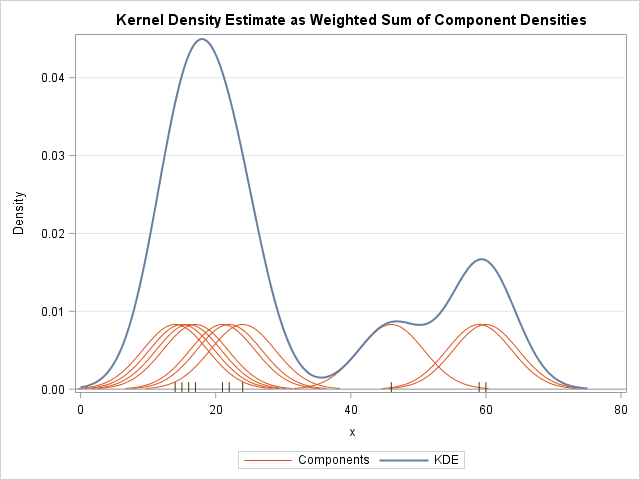https://blogs.sas.com/content/iml/2016/07/27/visualize-kernel-density-estimate.html

Different kernels can be used to obtain $p_n(x)$. Some very used examples are given below:

• Gaussian: $K(x) = \frac{1}{\sqrt{2 \pi}} exp\{ - \frac{x^2}{2} \}$
• Uniform: $K(x) = \frac{1}{2}I(-1\leq x \leq 1)$
• Epanechnikov: $K(x) = \frac{3}{4}max(1-x^2,0)$

As a rule of thumb, the use of Epanechnilov provides the lowest MSE. But this should be evaluated for each case. A non-exhaustive list of kernels is provided here.

Bandwidth selection

The exogenous parameter $h$ is the bandwidth of the kernels. It indicates how narrow are the kernel distributions around each sample point. Figure below shows the effect of $h$ in the final distribution $p_n(x)$. 

https://deepai.org/machine-learning-glossary-and-terms/kernel-density-estimation

In order to determine the optimum value for $h$, one should obtain the lowest possible MSE with respect to the true probability distribution:

$MSE = \frac{1}{4}|p''(x)|^2 \mu_K^2 + \frac{1}{nh}p(x)\sigma_K^2 + O(h^4)+O(\frac{1}{nh})$

where $p(x)$ is the "true" probability density obtained for the case in which $n \rightarrow N$ and $N$ is the population size, $\mu_K = \int y^2 K(y) dy$, and $\sigma_K = \int K^2(y) dy$. The optimum value $h_{opt}$ is then given by a minimization problem which results in:

$h_{opt} = \left(\frac{4}{n}\frac{p(x)}{|p''(x)|^2}\frac{\sigma^2_K}{\mu^2_K} \right)^{\frac{1}{5}}$
As described by equation above, for smooth valued $p(x)$ one might rely on narrow bandwidth. Otherwise, for distributions with more pronounced peaks, larger bandwidth values are more reliable. Evidently, if an analyst is interested in the use of kde is because she does not have the so-called "true" probability density $p(x)$ beforehand. In fact, the determination of $h_{opt}$ is a research topic. Here is an interesting paper handling this issue.
From a practical point of view, a well-established method relies on the use of estimators and optimization. An example is the Least-Square Cross Validation (LSCV) (this paper presents a good description). In this method, consists in finding the minima of the following expression:
$LSCV(h) = \int p_n^2(x, h) dx - \frac{2}{n} \sum^n_{i=1}p_{n, -i}(X_i, h)$
where $p_{n, -i} = \frac{1}{n-1}\sum^n_{j=1, j \neq i}\frac{1}{h}K\left( \frac{x-X_i}{h} \right)$ is the leave-one-out probability density estimation.
The estimator given by equation relies on an iterative method that remove the individual contribution of $X_i$ successively for all elements of the sample (cross-validation) and calculates the associated error with respect to complete case. The goal is to obtain a value of $h$ that provides the smallest estimator value. It is worth mentioning however that $LSCV(h)$ might have multiple minima which is problematic from the computational point of view since auxiliary or more complex optimization algorithms are required.

Certainly, this is not a complete discussion but I wanted to give just a brief overview of the method. Hope you enjoyed the post. Leave your comments and share.

Peace Profound and may the Force be with you.

#=================================

Diogo Pedroso

LinkedIn: www.linkedin.com/in/diogomourapedroso